This article will help you get introduced to yet another Conditional Formatting feature which will add more visual appeal to your reports. Instead of using CF we will make use of AutoShapes to determine a change in cell values. To accomplish this, let’s look at the below steps and screenshots:
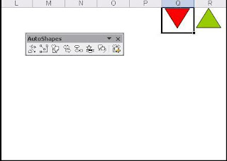
1) Open Microsoft Excel and go to Insert -> Picture -> AutoShapes. Choose Basic Shapes and select Isosceles Triangle from the list (You can choose the shape of your choice). Select a cell and draw the shape in that cell (I have merged 3 cells and accommodated the shape) and rotate the shape of the Triangle if you want. Right click on the Triangle, select Format AutoShape and under the Fill section choose the color of your choice which in my case happens to be Red. Copy the Red Triangle, paste it in another cell and change the color of the shape to a different color. So now I have 2 shapes in Red and Green. Look at the screenshot.
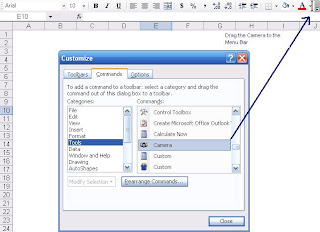
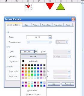
2) Next you need to go to Tools -> Customize and select Tools on the Left to view the goodies in the right section. Choose the Camera tool from this list and drag it to the Menu bar. Now select the cell with the AutoShape and click on the Camera icon. Start drawing the shape again and you will find a replica of the AutoShape you first created. Then as you can see in the screenshot, right click on the newly captured AutoShape and choose Format Picture. In the Colors and Lines tab, choose the No Fill and No Line options from the Fill->Color and Line->Color drop downs respectively. This will get rid of the outer boundary of your captured AutoShape. Have a look at the screenshots below to follow the steps.
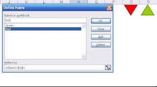
3) Then we need to name our 2 AutoShapes which we can do by going to Insert-> Name-> Define. Once there, we need to define the cells where the 2 Shapes are placed. In my case, I have referenced the cells and named them according to the color of the Shapes. This step is really crucial because we uniquely define the Shapes as these are the definitions by which we will be referencing them.
4) Now let’s look at the final step which deals with the definitions of the Alerts. First we have to define the cell where we will be displaying the number with name ‘Score1’ and statement = IF(Cell-value>5, 2, 1). The simple IF statement in the example validates the condition which in this case means if number is greater than 5 then choose 2 else choose 1. Finally we need to define the Alert which will be displayed next to the number validating the condition. Please look at the Step 4a image which shows that we have defined the Alert1 with the formula =Choose(Score1,Red,Green). This formula is helpful in providing an alias for the numbers used in the previous IF statement. So 1 means Red and 2 means Green.
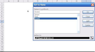
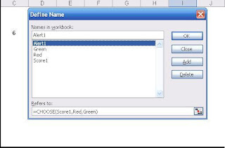
5) Now if we change the values in Cell C3 to a number lower than 5, we will see the Alert as Red and vice versa. Please look at the final 2 images which will give you an idea as to how these changes will take effect.
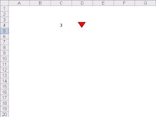
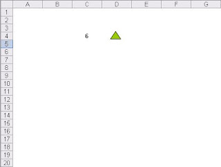
You can also download this file here. I hope you like this post as I think it was a refreshing change from the usual topics.
4 comments:
I tried your methods but do not get the same result. Are you skiping over steps? Where did the originial two autoshape screen captures go?
Thanks for your post. Very helpful
Hi,
I am not getting step 4, i did it as per what's given in your article. After having defined the cells and when i enter a figure in Score1, nothing happens.
Is there something that i missed out.
Would really appreciate your response.
Thanks alot
Priya
Hello Joshua/Priya,
I have posted a link to the actual Excel file. This should answer your questions.
I had the same problem, you have to select your copied picture and add =Alert1 in the formula bar. Then the picture will change based on the value of Alert1 which is based on the score.
Post a Comment